Quick Start¶

This page is a demo for quick usage once you have setup the environment dependencies.

Model Training¶

Codes in trainModel.py.

from ModelTrain import ModelTrain
from DataLoad import loadData
from util import *
from config import parser


def main():
   args = parser().parse_args()

   ## dataset path
   args.modelname = 'CH4_demo'
   args.input_path = os.path.join('Data', 'CH4_input.npy')
   args.label_path = os.path.join('Data', 'CH4_input.npy')

   ## mechanism file path
   args.mech_path = os.path.join('Chem', 'gri.yaml')

   setup_current_time(args)
   setup_device(args)
   create_model_path(args)
   setup_logging(args)
   train(args)


if __name__ == '__main__':
   main()

def train(args):
   input_train, label_train, input_valid, label_valid, norm = loadData(args)
   logging_args(args)  ## print hyper-parameters in log file
   model = ModelTrain()
   model.buildModel(args)
   model.trainingEntrance(input_train, label_train, input_valid, label_valid, args, norm)

You need to configure three basic hyper-parameters: modelname , data_path and mech_path , and then define the rules for data cleaning and pre-processing in DataLoad.py . Run the command :

python trainModel.py

Then DNN training starts. See .log files in /Model/model_name/log/*.log or loss curve in /Model/model_name/lossfile/*.png.

The default device for training is cuda:0, change the device via :

python trainModel.py --device 'cuda:1'

Change DNN hidden layers :

python trainModel.py -l 800 400 200 100

Add descriptions about your experiment purpose or motivation.

python trainModel.py -note 'validate my good idea.'

Model Usage¶

Use a trained DNN to perform prediction tasks. See codes in useModel.py.

Single-step prediction plots¶

from ModelUse import ModelUse
import numpy as np
import os

def main():
   modelname = 'CH4_demo'
   epoch = 5000
   mech_path = os.path.join('Chem', 'gri.yaml')
   input='Data/GRI3CH4/X_134w_AdapManCH4_constP.npy'
   label='Data/GRI3CH4/Y_134w_AdapManCH4_constP.npy'
   data_name='134w_AdapManCH4_constP'
   oneStepPred(modelname,epoch,mech_path,input,label,data_name,plot_dims=[0,2,3,4,5,6])

if __name__ == '__main__':
   main()

def oneStepPred(modelname,epoch,mech_path,input,label,data_name,plot_dims):
    model=ModelUse()
    model.initGas(mech_path)
    model.loadModel(modelname,epoch)
    model.oneStepPredict(modelname,epoch,input,label,data_name,plot_dims,dpi=200)

Set modelname and epoch determining which checkpoint to be loaded. Choose the mechanism input file mech_path for Cantera. Then configure the path of testing dataset input and label. Run the command :

python useModel.py

See the figures saved in /Picture/OneStepPred/ e.g.

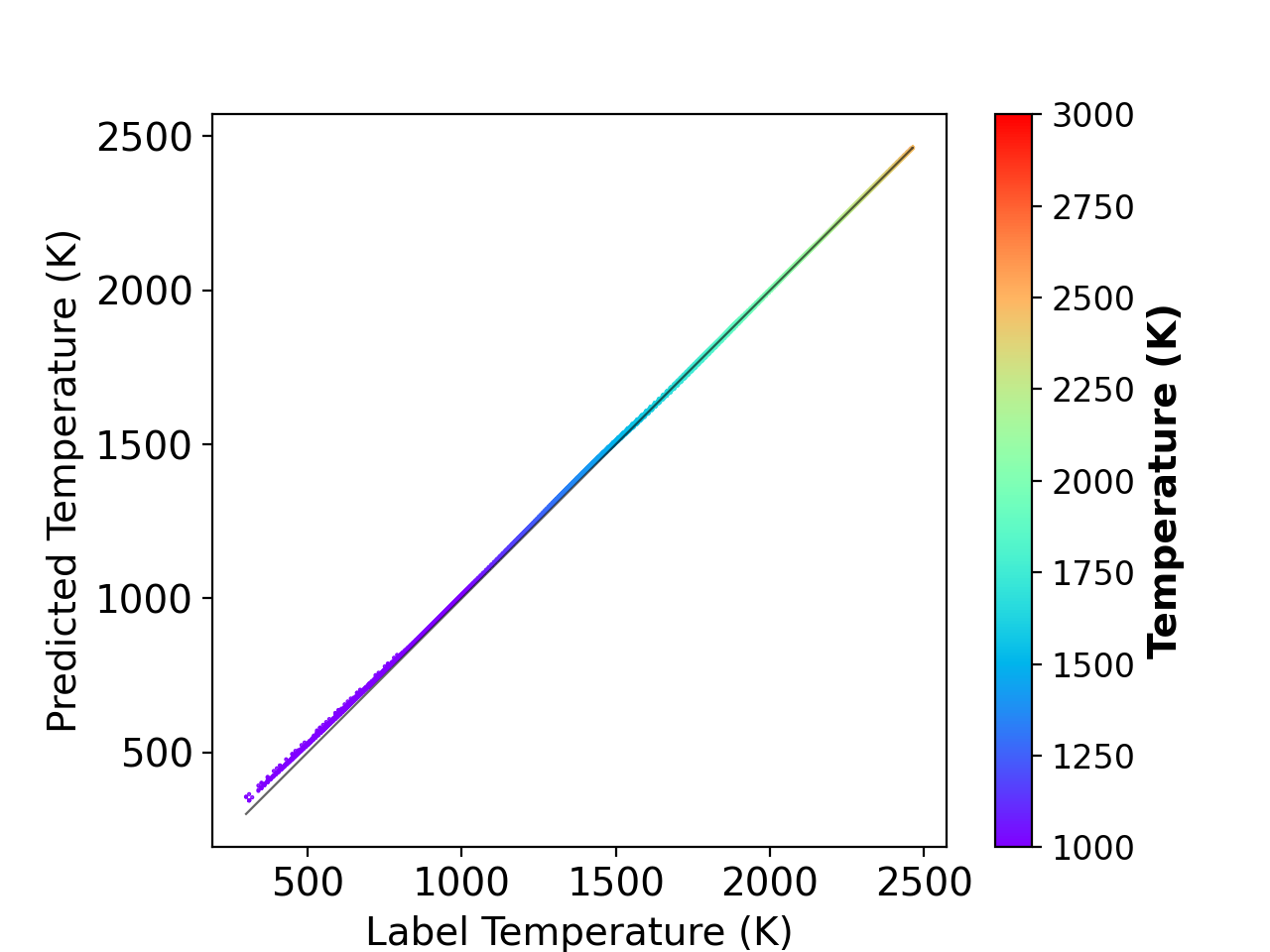
../_images/Methane_GRI3.0_134wAdapManCH4constP_2022-07-31_epoch5000_OneStepPred_on_1.7w_1dFlameCH4_constP_dim=0.png — Fig 1 : Single-step prediction on the testing dataset.

Temporal evolution¶

from ModelUse import ModelUse
import numpy as np
import os

def main():
   ## modelname
   modelname = 'CH4_demo'
   epoch = 5000
   ## mechanism path
   mech_path = os.path.join('Chem', 'gri.yaml')

   n_step=5000 # dnn interation steps
   builtin_t=1e-8 # cantera max time step

   gas_condition=[phi,1600,1,'H2','constP'] # Phi,T,P(atm),fuel,reactor
   temporalEvolution(modelname,epoch,mech_path,gas_condition,n_step,builtin_t)

if __name__ == '__main__':
   main()

def temporalEvolution(modelname,epoch,mech_path,gas_condition,n_step,builtin_t):
    model = ModelUse()
    model.initGas(mech_path)
    model.loadModel(modelname,epoch)
    model.evolutionPredict(modelname, epoch, gas_condition, n_step, builtin_t, plotAll=0, dpi=200)

Set modelname and epoch determining which checkpoint to be loaded. Choose the mechanism input file mech_path for Cantera. Setup initial conditions for auto-ignition and then run :

python useModel.py

Check /Model/modename/pic/ for temporal evolution plots.

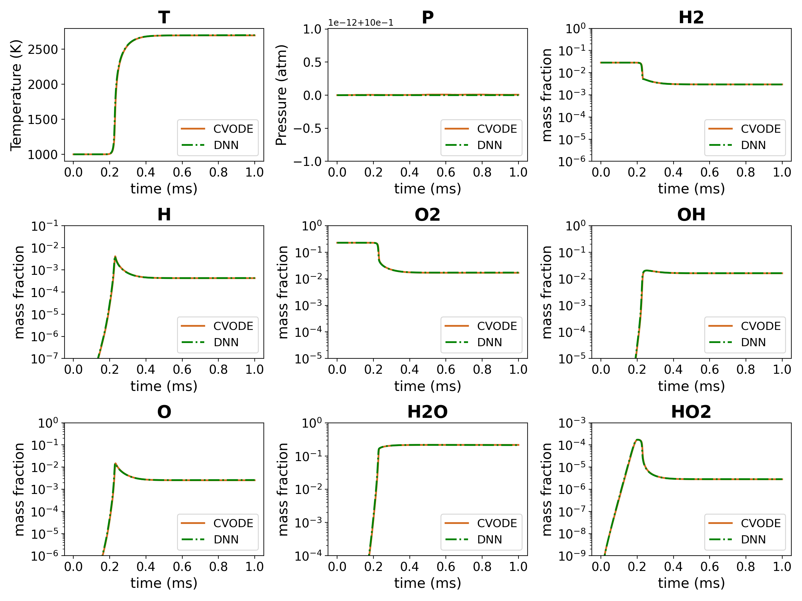
../_images/820w_mmsH2_constP_Phi=1_T=1000_P=1_epoch=5000_all1.png — Fig 2 : Temporal evolution of hydrogen/air mixture.

Visualization¶

Draw the distribution and phase diagram of chemical dataset. See codes in plot.py

Distribution¶

import sys,os
import matplotlib.pyplot as plt
import seaborn as sns
from VisualArt import VisualArt
import numpy as np

Plotter=VisualArt()
mech_path='Chem/H2_12s.yaml'
Plotter.initGas(mech_path)

scale='log'

input_path = 'Data/X_810w_mmsH2_constP.npy'
data_name = '810w_mmsH2_constP'

Plotter.singleDisplot(input,data_name,scale,plot_dims='all')

Run the command :

python plot.py

Then check the distribution plots of the given dataset in /Picture/Distribution/.

../_images/displot_of_900w_mmsH2_constP_1_scale=log.png — Fig 3 : Distribution of a hydrogen dataset.

Phase diagram¶

import sys,os
import matplotlib.pyplot as plt
import seaborn as sns
from VisualArt import VisualArt
import numpy as np

Plotter=VisualArt()
mech_path='Chem/H2_12s.yaml'
Plotter.initGas(mech_path)

input = 'Data/X_810w_mmsH2_constP.npy'
label = 'Data/Y_810w_mmsH2_constP.npy'
data_name = '810w_mmsH2_constP'

Plotter.phaseDiagram(input,label,delta_t,data_name,size_show=500000)

Run the command :

python plot.py

Then check the phase diagrams of the given dataset in /Picture/PhaseDiagram/.

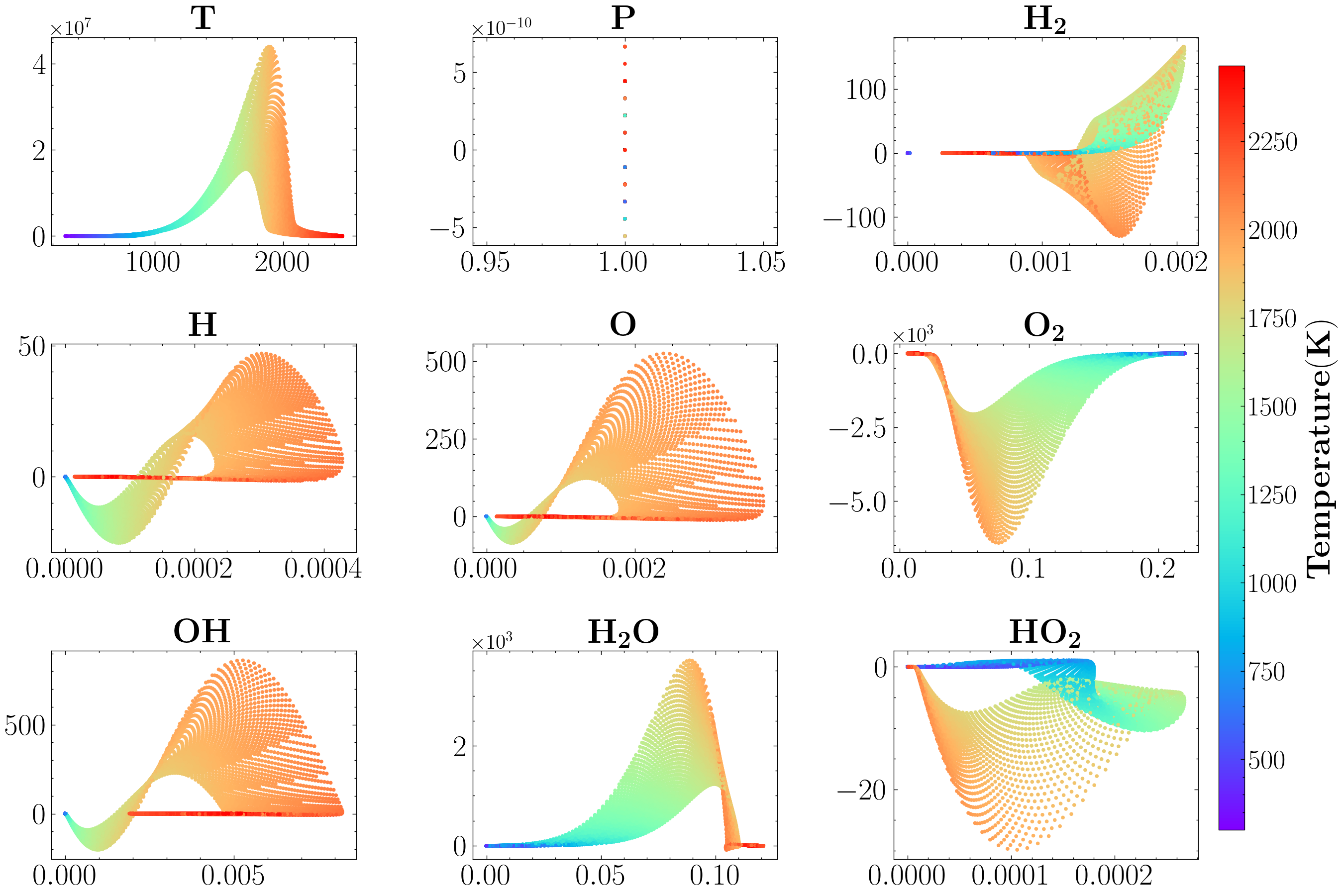
../_images/phase_of_1.7w_1dFlameCH4_constP_1.png — Fig 4 : Phase diagram of methane one-dimensional flame.

Sampling Methods¶

Sampling methods